CAPAREDA CURVE

| next curve | previous curve | 2D curves | 3D curves | surfaces | fractals | polyhedra |
CAPAREDA CURVE
| Curves studied by Levi Capareda in 2010. |
The Capareda curves are the curves traced
on a sphere the projection of which on an equatorial plane of the sphere
is a hypo-
or epi-trochoid
inscribed in the equator. In fact, they are precisely the same curve, with
a different presentation, as the satellite
curves.
Cartesian parametrization in the case of the hypotrochoid:
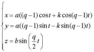 with
with In the case of the epitrochoid:  with
with |
Case of the hypotrochoid:
For k = 0, we get the equatorial circle (or a
cylindric
sine wave for any choice of b).
For k = q 1, we get the clelias
of index  > 1 (case where the poles are multiple points; the equatorial projection
is a rose).
> 1 (case where the poles are multiple points; the equatorial projection
is a rose).

|
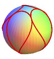
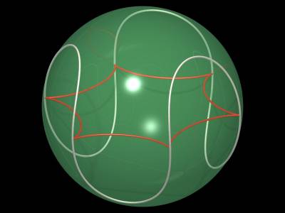
q = 6, k = 1 |
q = 4, k = 3 (clelia) |

q = 4 , k = 1 (seam line of a tennis ball) |
q = 3, k = 2 (clelia) |
q = 3, k = 1 |
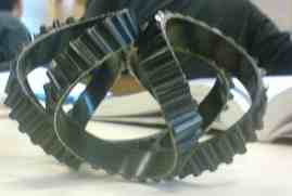
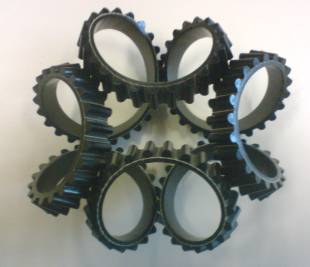
| Case q = 8, k = 4,3 modelled by Levi Capareda with a gear belt during an Industrial Sciences lecture... |
 |
 |
 |
 |
Case of the epitrochoid:
For k = 0, we get the equatorial circle (or a
cylindric
sine wave for any choice of b).
For k = 1, we get the spherical
helices.
For k = q + 1, we get the clelias
of index  < 1 (case where the poles are multiple points; the equatorial projection
is a rose).
< 1 (case where the poles are multiple points; the equatorial projection
is a rose).
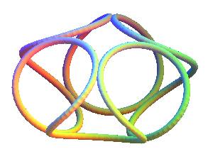
q = 4, k = 1 (spherical helix) |

q = 4, k = 2 |
q = 4, k = 5 (clelia) |
q = 6, k = 7 |
.jpg)
.jpg)
.jpg)
.jpg)
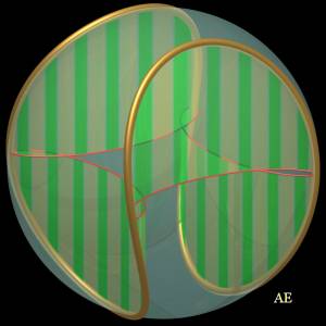
Some examples with the equatorial projections, by Alain Esculier
| next curve | previous curve | 2D curves | 3D curves | surfaces | fractals | polyhedra |
© Robert FERRÉOL 2018