Curve studied by Cassini in 1680 and Malfatti in 1781. Informal name: cat eyes. Jean-Dominique Cassini (1625-1712): French astronomer. Excerpt from Éléments d'astronomie by Jean Cassini (1740): Since the exact observation of the apparent length of the diameters of the Sun, my father has found a new curve, different from the ellipse, that can represent very precisely the true movements of the Sun and its various distances from the Earth. He assumes that the Earth being on one of the foci of the curve, the Sun describes it in its proper motion in such a way that if you draw two lines from the centre of the Sun to the two foci of the curve, the rectangle defined by these lines is always equal to the rectangle defined by the larger and the smaller distances between the Sun and the Earth.  Excerpt from l'Encyclopédie by d'Alembert, T. 1 page 633 (1784): This curve, that Mr Cassini had wished to introduce in Astronomy, is now only a purely geometric curve and an object of curiosity, because we know that planets describe Apollonian or ordinary ellipses. One may ask why Mr Cassini substituted this ellipse to Kepler's. Here is my conjecture on the subject. It is known that most of the planets describe ellipses with low eccentricity. It is also known that in an ellipse with low eccentricity, the angular sectors created by vector rays from a focus are almost proportional to the corresponding angles at the other focus, and it is thanks to this property that Ward gave the approached solution of the problem that consists in finding the true anomaly of a planet, the mean anomaly being given. The ratio between the infinitely small sector and the corresponding angle is like the rectangle of two lines passing through the focus, and in an ellipse with low eccentricity, this rectangle is almost constant: this is Ward's principle. Yet, Mr Cassini seems to have reasoned like this: since the ratio between elementary sectors with corresponding angles is like this rectangle, it will be constant in a curve where the rectangle is constant. Therefore, he imagined the cassinoid.

 

Bipolar equation:  , the pole O being the middle of the two foci , with . Cartesian parametrization: 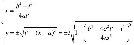 (t = r); for the component on the right when ,  when . Polar equation:  i.e., with , , the equation with " – " yielding real points only when e1 , with . Cartesian equation: , or , or  or even:, for . Elliptic bicircular quartic (rational for e = 1). 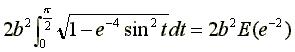Radius of curvature: . The inflection points are therefore located on the lemniscate (in green opposite) :  Area for e1: (E = elliptic integral of the second kind). Area of an oval for e < 1: (K = elliptic integral of the first kind).

The Cassini ovals are the loci of the points on the plane for which the geometric mean of the distances to two points, the foci, is constant (= b).
They also are the field lines of the vector field 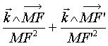, sum of two orthoradial 1/r fields.

In the case when e < 1 (b < a), the "oval" is composed of two curves shaped like symmetrical eggs with respect to O with tripolar equations:

 where, .

In this case, the curve is anallagmatic: invariant under the inversion of centre O and radius   ; therefore we have a cyclic generation: the initial curve is the hyperbola 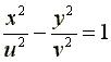 with 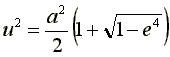 and , and the inversion circle (with radius Öp) is the Monge circle.

The Cassini oval as the envelope of the circles centred on a hyperbola and orthogonal to its Monge circle.

Case e = 1 (b =  a): it is the lemniscate of Bernoulli (here )

In the case when e > 1, the real Cassini oval is no longer anallagmatic, but the complex curve still is, with a complex inversion radius.

For  (): the oval has the shape of an "ellipse" that is worn out at the summits of the minor axis.

For , the oval finally has an oval shape. Valery Ochkov proposes to baptize it "oval of Tolstoy" for its resemblance with
Tsarskoye Selo hippodrome near Saint Petersburg, hippodrome mentioned in the novel "Anna Karenina".

For (): the oval finally has an oval shape, leaning towards a circular shape as e increases to infinity.

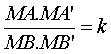In the case when e < 1, the equation  can be written , where   and 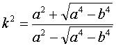(Wangerin's theorem link page 19).

The Cassini ovals also are the sections of a torus by planes parallel to the axis, located at a distance to the axis equal to the minor radius of the torus (here, section of a torus with major radius R = a and minor radius   by a plane located at distance r to the axis - the torus is thus a spindle torus for ) ; see spiric of Perseus.
 

The field lines of the magnetic field created by two parallel wires carrying currents of equal intensity in the same direction are, in any plane orthogonal to the wires, the Cassini ovals with foci the intersection points with the wires. The same is true for the equipotential lines of the electrostatic field created by two uniformly charged parallel wires with identical charge.

The orthogonal trajectories of the Cassini ovals are the rectangular hyperbolas with polar equation 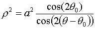  ; they are the electrostatic field lines in the physical interpretation above.

If, in the definition of the Cassini ovals, the geometric mean were replaced by the arithmetic mean, it would result in ellipses, and if it were replaced by the harmonic mean, it would yield Cayley ovals.

See the generalisation that are Cassinian curves, also compare with Booth curves and look at surfaces of Cassini.

next curve

previous curve

2D curves

3D curves

surfaces

fractals

polyhedra

© Robert FERRÉOL 2017